Understanding Local LLM Inference

What is inference?

Training is the process by which a model learns its weights. Inference is everything after, once the model is built, you give it a prompt and it produces output. When you run a model locally, you are only doing inference, the weights are already baked in.

A language model generates text one token at a time, and it is autoregressive, so each token it produces gets fed back in as part of the input for the next one. A 500-token reply means 500 sequential passes through the network, each one conditioned on everything before it. The reason why you cannot receive instant responses is because Token N+1 cannot start until token N exists.

When you are talking to the model, inference is memory-bound, not compute-bound. The GPU spends most of its time waiting to read the model's weights out of memory. This is the opposite of training workloads, where the computational operations are the main bottleneck. As a result, available memory bandwidth often have a greater impact on token generation speed than raw FLOPS.

Quantisation

Think of a model's weights as just numbers (because they are). Most trained models store each weight as a 16-bit float (FP16), two bytes each. Quantisation stores them at lower precision instead: 8 bits, more commonly 4, sometimes less.

Quantisation is essentially a trade-off between accuracy and efficiency. By reducing weights to 4 bits, you compress the model by storing a simplified version of the original values. This introduces a small loss in precision, which can slightly affect output quality, but the reduction in memory usage is significant. Since inference is usually constrained by how quickly data can be moved from memory, the smaller model size can also increase generation speed. This makes quantisation one of the key techniques for running large models efficiently on local hardware.

In the GGUF ecosystem, models are available in a range of quantisation levels, with formats such as Q8, Q5_K_M, Q4_K_M, and Q3_K_S and down. Q4 is often considered the best balance between size and quality. Higher precision formats consume considerably more memory while providing improvements that many users will not notice. Lower precision formats save more space but can introduce more noticeable quality loss, with the model becoming less coherent, more repetitive, or struggling to maintain context.

VRAM Usage

Three things determine whether a model fits on your GPU or not. Although there are a number of preset calculators to see if a model can run on your GPU, the main three things that use VRAM are:

• The weights are the largest part and the easiest to estimate. For a Q4 quantised model, a useful approximation is around 0.5GB of VRAM per billion parameters. This means a 7B model will typically need around 4GB, a 13B model around 8GB, and a 70B model more than 35GB.
• The KV cache stores intermediate state for every token in the context so it does not recompute the whole history each step. The size of this cache increases with the context length, meaning long conversations or large documents can consume several additional gigabytes of VRAM. If a model loads successfully but runs out of memory later during use, the KV cache is often the cause.
• There is also some additional VRAM usage from activations and the inference runtime. This is usually much smaller, but it is important to leave some headroom rather than using the entire capacity of the GPU.

As a rough estimate, take the parameter count, halve it to estimate Q4 memory usage in gigabytes, then add a few extra gigabytes for context and overhead. If the total fits within your GPU's VRAM, the model should run comfortably.

Context windows

The context window is how much text the model can attend to at once, including prompt and output, measured in tokens. As mentioned above, the KV cache grows linearly with context length, so doubling your context roughly doubles that memory. For short inputs this overhead is not noticeable, but with very long contexts it becomes a major factor in both memory use and speed. A good approach is to only use as much context as the task requires. Providing large amounts of text such as full codebases when it is not necessary increases memory and compute costs without any benefits.

Reading benchmark numbers

Inference has two stages:

• Prefill is the phase where the model processes the input prompt and builds its internal state. This step runs over all input tokens at once, which allows more parallelism. The main observable metric is time to first token, which is the delay before any output appears. This phase is compute-bound.
• Decode is the generation itself, the token-by-token part. This is the memory-bound phase, and it is what tokens-per-second measures, e.g. how fast text streams out once it has started. This phase is memory-bound.

So a model can have a quick time-to-first-token and slow tokens-per-second, or the other way round, and a single value does not mean anything on its own, as a benchmark should quote both, because they measure different speeds. Prefill is how long until it responds, decode is how fast it talks.

The tradeoff triangle

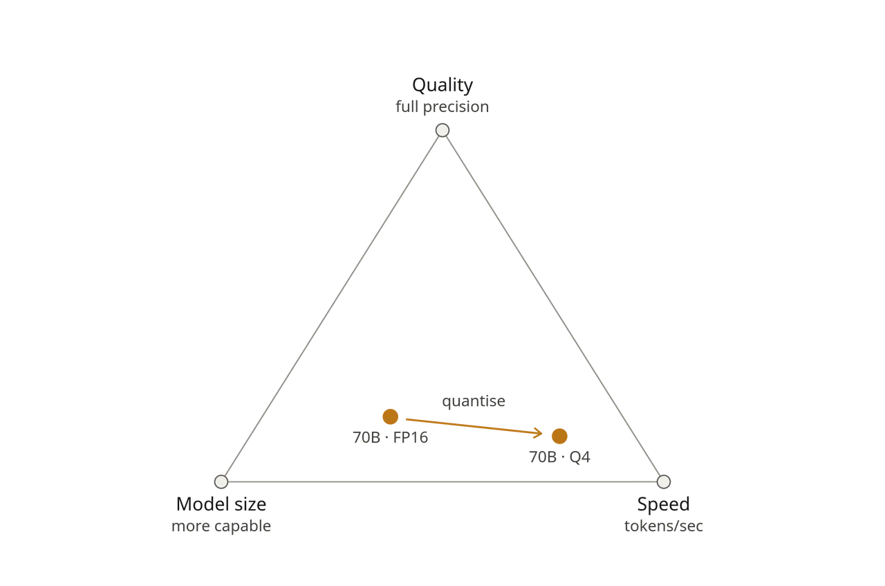There is always a trade-off and you cannot max everything out on fixed hardware, as these three things pull against each other:

• Model size: bigger models are more capable.
• Speed: smaller and more quantised models run faster.
• Quality: full precision keeps the model's trained ability.

Quantisation shifts the balance between these factors. It reduces memory usage and often increases throughput, at the cost of some reduction in accuracy. On systems with limited VRAM, this trade-off determines what can run at all.

The usable configuration is the one that fits within memory limits while still meeting latency requirements. A smaller model that runs consistently is much better than a larger model that cannot be loaded or is too slow to use interactively.

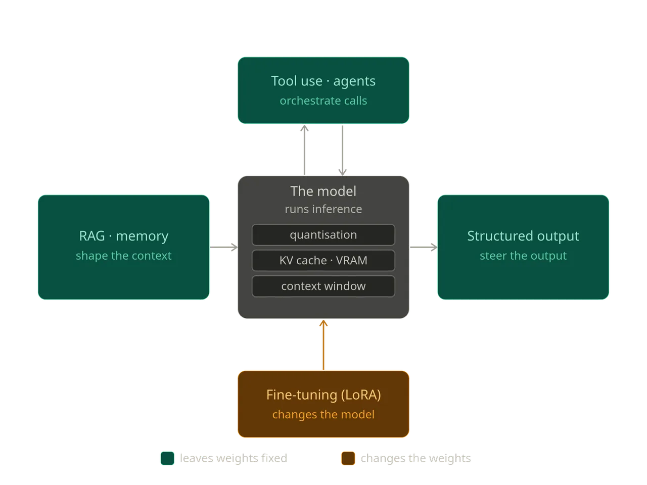
Architectural Patterns

The mechanics described earlier assume a single model running as a fixed unit, with weights loaded in memory and tokens generated sequentially. Architectural patterns operate around that unit.

They do not alter the inference process itself, but they influence the input provided, the structure of the output, and how multiple model calls are coordinated.

A useful way to separate them is by their point of interaction. Some modify or structure the context sent into the model. Others shape or constrain the output it produces.

Retrieval-augmented generation (RAG)

A model can only use information that is present in its current context, and that context is limited in size and cost. RAG avoids loading everything at once, instead of placing large amounts of data into the prompt, external data is stored separately and only relevant parts are inserted at query time.

The inference process remains unchanged, but it makes a difference in how the input context is constructed.

RAG commonly uses a vector database, where text is converted into embeddings, and retrieval is based on similarity to the query. Another approach is a knowledge graph, where data is accessed by traversing defined relationships rather than similarity search. Both methods aim to reduce the amount of irrelevant information sent to the model.

With RAG, the retrieval quality is determined by embedding generation, chunking strategy, hybrid search, and graph traversal. So if context size is a limitation, RAG is the way to go.

Memory

Memory can be viewed as RAG applied to the system’s own interaction history. Instead of retrieving from an external knowledge base, it retrieves from prior conversations, session history, or user-specific data. The underlying mechanism is similar, using embedding, storage, and retrieval, but the purpose and update pattern differ because memory is written continuously rather than preloaded.

It is typically split into short-term memory, which is the active context window of the current session, and long-term memory, which is stored externally and reused across sessions. A common further distinction is between episodic memory, which records specific events such as past interactions, and semantic memory, which stores stable preferences or facts like units or formatting choices.

Without memory, the system remains stateless even if individual responses are coherent. Persistent storage of prior interactions is what enables continuity across sessions.

Structured output

By default, models generate free-form text, which works for chat but is unreliable for machine consumption. Structured output constrains responses into defined formats such as JSON, schemas, or grammars. The basic approach is prompt-based instruction, which is not fully reliable. On a large scale system, you can use constrained decoding, where token selection is restricted at generation time so that only valid sequences under a schema are allowed. In implementations like llama.cpp this is handled with GBNF grammars.

Tool use

Tool use allows a model to trigger external functions instead of only producing text. A tool is defined as a function interface, and the model outputs a structured call request. External code executes the function and returns the result to the model as part of the context.

The model does not execute tools directly. It only selects and formats the call. Reliability depends on structured output, since tool calls must be valid and machine-readable. This pattern enables integration with external systems such as search, databases, or IoT devices without changing the model itself.

Agent loops

Agent loops extend tool use into repeated cycles. The model is run in a loop where it interprets a goal, selects an action, observes the result, and continues or stops based on the updated state. This allows a model to perform multi-step tasks rather than single responses. The main complexity is not the loop itself but control logic, including termination conditions, error handling, and preventing repetitive / divergent behaviour.

Fine-tuning

Most of the earlier approaches keep the base model unchanged and work around it. Fine-tuning changes the model itself, as a pretrained model is trained further on additional data so that its weights shift toward a specific domain, style, or output format.

Full fine-tuning is extremely resource intensive, so local setups use alternative methods like LoRA or QLoRA. These approaches keep the original weights frozen and train smaller adapter layers instead. This reduces memory and compute requirements enough to make training feasible on consumer GPUs.

Fine-tuning is mainly useful for controlling the overall behaviour and output structure. It is effective for consistent formatting, tone, or task-specific patterns. It is not well suited for injecting factual knowledge, though. The learned information is fixed at training time, and updating it requires additional training. This separates it from RAG, since RAG is used when information needs to be current or changeable, since it retrieves data at inference time. Fine-tuning is used when the goal is stable behaviour rather than external knowledge.